How to Translate Only Selected Text in Excel Spreadsheets


I assume you someties work with large Excel spreadsheets that have a lot of numbers and only a few text columns to translate.
To translate them, you can simply cut and paste the columns that need translation into a separate file. After translating, you can then copy and paste them back into your original file.
But wait—we’ve got a simpler option for you!
You can hide the columns you don’t need to translate and use your preferred CAT tool to translate the remaining visible columns.
To do that:
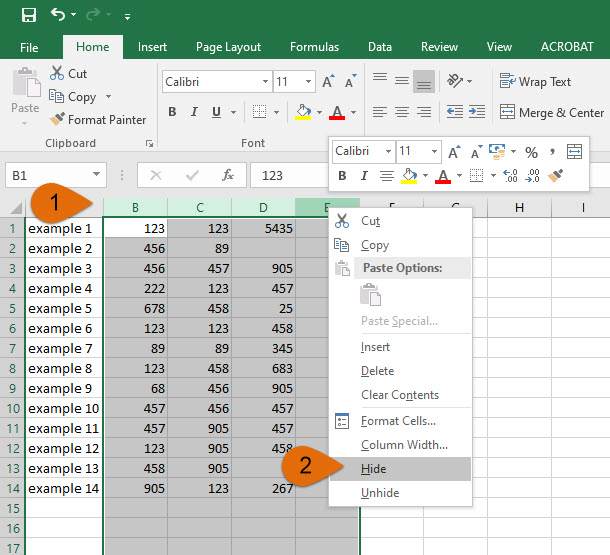
1. Select one or more columns. If you need to select any additional, nonadjacent columns, press Ctrl.
2. Right-click the selected columns and press the Hide command (see the screenshot below). Instead of each hidden column, you will see the double line between the adjacent columns.
If you don’t see the command in the right-click menu, you can locate it in your editing ribbon, in the Home tab by opening the Format menu (under Cells). In the dropdown menu, locate the Visibility section, click the Hide & Unhide command, and select the appropriate Hide Columns option.
3. Complete the translation and generate the target Excel file. Before finalizing your project, make sure to unhide the hidden columns!
To unhide each column, first select the adjacent columns and right-click to select Unhide. (If the right-click menu does not display that command, you can find it in the same Format menu, as we have explained before.) Or you can simply double-click the double lines between the adjacent columns where each hidden column is located.
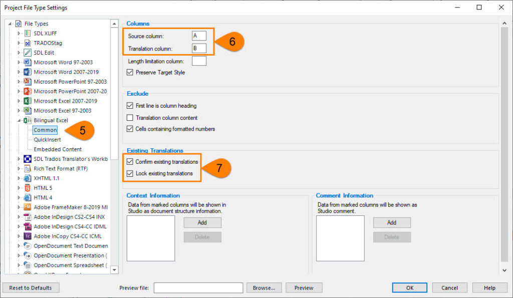
When translating, make sure to appropriately set your CAT settings so that the program does not translate any hidden text. In SDL Trados, for example, when specifying the Project Settings, go to the File Types menu and, under the file type of Microsoft Excel, select the Common tab to uncheck or disable the Hidden Content option (see the screenshot below).
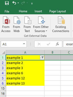
For other projects, you may need to translate other selective parts in the file. For example, you may need to translate only the cells that are highlighted in yellow:
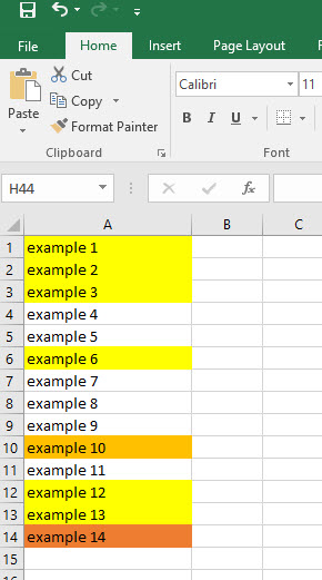
To translate only the highlighted cells in a column, do the following:
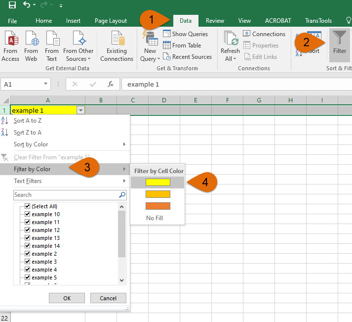
- Select the first row of the column.
- Open the Data tab in your editing ribbon and click Filter.
- You will notice a dropdown button appear in the lower right corner of the first cell. Click on the arrow on the button.
- From the dropdown menu, select Filter by Color.
- Select the highlight color.
After you make a selection, only the color you chose will appear on the spreadsheet; all other cells will be hidden.
To translate the selected text:
- Save your file, which now displays only the highlighted cells.
- Create a project in your CAT tool and complete the translation.
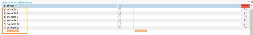
- Generate the target translation.
- To unhide the hidden content in your newly translated Excel spreadsheet, deactivate the filter. To do that, click Data > Filter, or use the keyboard shortcut Ctrl-Shift-L.
Your file, with the translated and other content, is ready for delivery!
Did you find these tips helpful? Feel free to share them with your PMs. We bet this will come in handy!
Should you need our services, including DTP (InDesign, AutoCAD, Photoshop, Illustrator) and PDF > DOC conversion (CAT tool file preparation), let us know by replying to this email. We are looking forward to hearing from you!